Stratified turbulence#
Few experimental results#
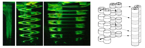
Fig. 6 (a) Photographies of the evolution of the zigzag instability of two columnar counter rotating vortices. The dipole propagates initially towards the reader. (b) Scheme of the non-linear evolution of the zigzag instability inllustrating the creation of pancake vortices. Taken from Billant and Chomaz [2000].#
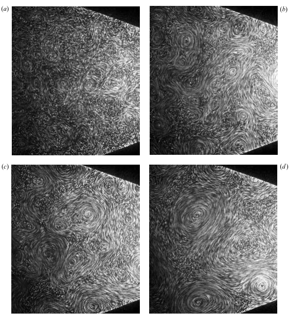
Fig. 7 Streak photographs of an evolving, grid-generated turbulent flow. Taken from Praud et al. [2005].#
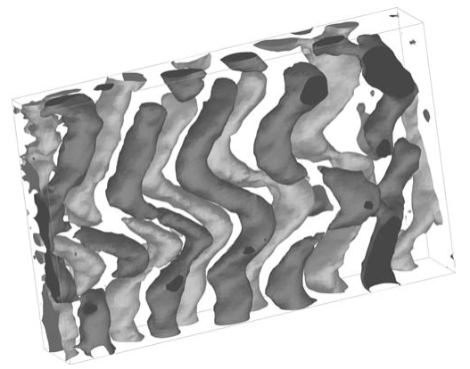
Fig. 8 Initial three-dimensional instability of the laminar wake represented in terms of isosurfaces of the vertical component of vorticity \(\omega_z\). Taken from Praud et al. [2005].#
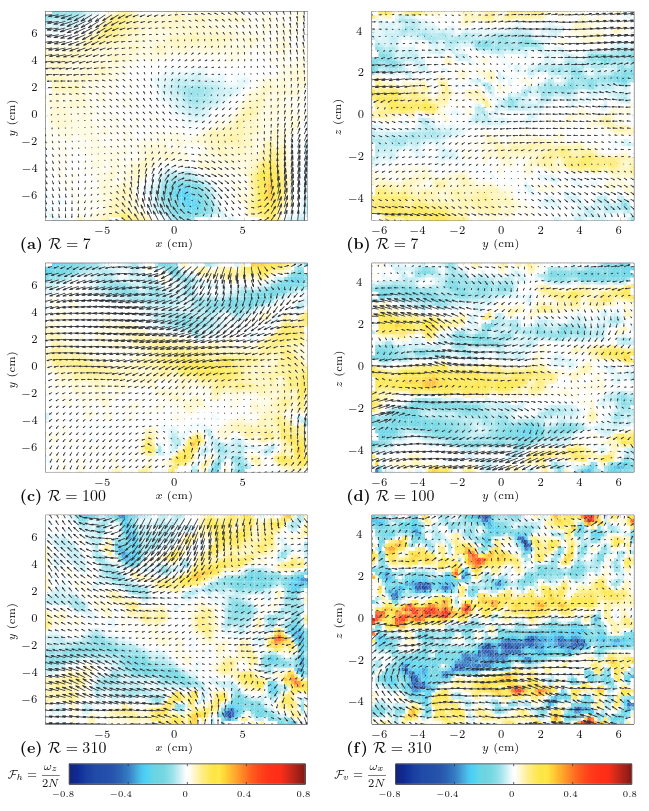
Fig. 9 Horizontal ((a), (c), (e)) and vertical ((b), (d), (f)) cross-sections of the velocity in the quasi-stationary regime for three values of the buoyancy Reynolds number \(\R\). Taken from Augier et al. [2014].#
Scaling analyses#
Inviscid stratified flows#
Let us follow Billant and Chomaz [2001] by considering a flow with typical horizontal velocity \(U\), typical horizontal scale \(L_h\) and typical vertical scale \(L_z\). We define the aspect ratio \(\alpha \equiv L_z/L_h\). The most important non-dimensional parameter is the horizontal Froude number \(F_h \equiv U / (N L_h) \).
We found the first two scaling laws. We can then compute the ratio
which implies that the two terms of the right hand side of the vertical velocity equation have to be of the same order, which gives:
We can rewrite the equation using the dimensionless variables:
with
Dominant balance gives \(\alpha\sim F_h \Rightarrow L_z \sim U/N\). This important scale is called the buoyancy scale \(L_b \equiv U/N\). This scaling implies that the potential energy is of the same order of magnitude as the kinetic energy.
Viscous stratified flows#
Brethouwer et al. [2007]
Using the strongly stratified scaling presented above, the diffusive equations are written in non-dimensional form as
where \(Sc = \nu / \kappa\) is the Schmidt number. If we only keep the dominant terms when \(F_h \rightarrow 0\), it yields
At this point, we need to define the buoyancy Reynolds number
where \(L_\nu = \sqrt{\nu L_h / U}\).
Small buoyancy Reynolds number limit
\(L_z \sim L_\nu\). Viscous stratified turbulence with 2D like advective term. Recover equations found by Riley et al. [1981] in the limit of \(Fr < 1\) (i.e. \(F_h < 1\) and \(F_v < 1\)).
Large buoyancy Reynolds number limit
\(L_z \sim L_b = U/N\), \(E_P \sim E_K\). Strongly anisotropic with a 3D like advective term.
\(\Rightarrow\) “Strongly Stratified Turbulence” regime, latter called LAST regime (Layered Anisotropic Stratified Turbulence).
Few numerical results#
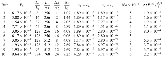
Fig. 10 Lindborg [2006] simulation parameters. \(No\) is the number of time steps and \(\Delta t\) is the time step in the statistically stationary state. For run 6 no stationary state was reached and the time step was therefore decreasing during the whole run.#
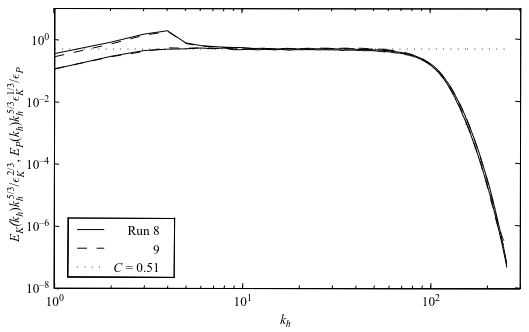
Fig. 11 Compensated horizontal kinetic and potential energy spectra from runs 8 and 9.#