Few observations in the atmosphere and the oceans#
Measurements in the atmosphere#
The velocity and temperature in the free atmosphere (high troposphere, stratosphere and mesosphere) can be measured by probes fixed on aircrafts, ballons or rockets, giving one-dimensional measurements. There are also LIDAR and RADAR measurements. Globally, the measurements are very sparsed.
Horizontal profiles#
From measurements of probes on aircrafts, one can compute signals as a function of an horizontal coordinate (Taylor approximation). The simplest quantity than one can compute from these signals are “horizontal spectra”. Figure Fig. 2 show 3 spectra of zonal wind, meridional wind and potential temperature.
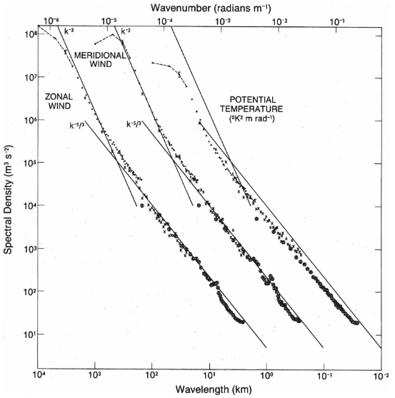
Fig. 2 From left to right, variance power spectra of zonal wind, meridional wind, and potential temperature near the tropopause from Global Atmospheric Sampling Program aircraft data. The spectra for meridional wind and temperature are shifted 1 and 2 decades to the right, respectively. Reproduced from Nastrom and Gage [1985].#
The \({k_h}^{-5/3}\) scaling low suggests an energy cascade but it cannot be related to standard isotropic turbulence since (i) the atmosphere is very shallow and (ii) the flows at such large scales are strongly influenced by rotation and stratification. We will present different interpretations of these spectra.
Observations indicate that the energy cascade is downscale at scales below 100 km (Lindborg & Cho 2001).
We will see that some decompositions (horizontal vorticity/horizontal divergence, geostrophic/ageostrophic) can be useful… But controversy (incompatible results):
Vertical profiles#
\({k_z}^{-2}\) at the largest scales, \({k_z}^{-3}\) at intermediate scales and shallowing towards \({k_z}^{-5/3}\) at smallest scale. See for example Fritts and Alexander [2003].
Measurements in the oceans#
Garrett & Munk (1975) produced an analytical models able to approximatelly describe oceanic spectra computed from measurements. Temporal and vertical spectra measurements are very common (fixed and dropped probes, respectivelly). Horizontal spectra are more difficult to measure (towed probes).
For the temporal spectra, the energy is concentrated at frequencies between \(f\) and \(N\), indicating that internal gravity waves are important.
Garrett & Munk model assumes that the spectra are only due to waves.
TODO: Lvov…
Vertical profiles#
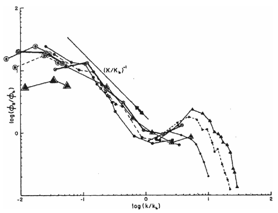
Fig. 3 Vertical wavenumber spectra of vertical shear in the ocean. The spectra are normalized by … and the wavenumber is normalized by \(k_o\). Reproduced from Gargett et al. [1981].#
Horizontal profiles#
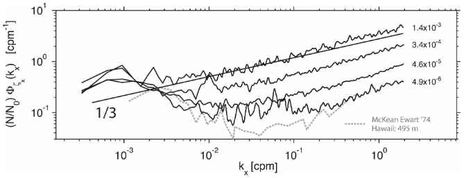
Fig. 4 Average isopycnal slope spectra, binned in one-decade bins of the turbulent diffusivity … and normalized by \(N_0/N\) (from Klymak and Moum [2007]). A line with slope \(k_x^{1/3}\) has been added for comparison. Taken from Riley and Lindborg [2008].#
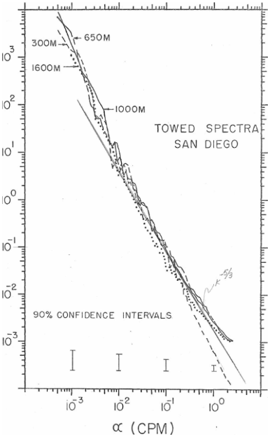
Fig. 5 Power spectra of temperature vs horizontal wavenumber \(\alpha = k_h\) computed from runs off the coast of San Diego (30°N, 124°W). The spectra are normalized by \(N/N_0G\), where \(G\) is the temperature gradient averaged over several measurements, and the buoyancy frequency \(N\) has been fitted to the exponential profile \(N = N_0 e^{z/b}\). The units of the spectra are m\(^2\)/cpm. Reproduced from Ewart [1976].#
Summary#
Horizontal spectra steep (\({k_h}^{-3}\)) at large scale and \({k_h}^{-5/3}\) at moderate scales (\(\sim\) 100 km in the atmosphere and \(\sim\) 5 km in the oceans).
Downscale energy cascade (Lindborg (1999); Cho & Lindborg (2001); Lindborg & Cho (2001)).
\({k_z}^{-2}\) at the largest scales, \({k_z}^{-3}\) at intermediate vertical scales and shallowing towards \({k_z}^{-5/3}\) at smallest scale.
Still contreverse about decomposition… Dominated by ageostrophic modes.
Different interpretations of the geophysical spectra#
Two “old” hypothesis#
Waves turbulence (Dewan [1979] for the atmosphere, Garrett & Munk 1975 for the oceans): downscale energy cascade
Stratified turbulence (Lilly 1983): upscale (inverse) energy cascade, similar to 2D turbulence, like quasi-geostrophique limit (potential enstrophy conserved and proportional to the energy in Fourier space).
Hopefully, these two very different interpretations lead to opposite predictions: wave theories predict a forward cascade, while vortex Lilly’s theory predicts a backward cascade.
The direction of the energy cascade in the atmosphere has been measured by Lindborg (1999); Cho & Lindborg (2001); Lindborg & Cho (2001). The third order structure functions are shown to be proportional to negative \(r\), where \(r\) is the separation distance, which implies a downscale energy cascade. This tends to show that the energy spectra can not be explained by a two-dimensional dynamics and thus gives credit to the wave theories that predict a downscale energy cascade.
More theories based on waves#
The concept of “wave saturation” has been used to explain the universality of the spectra (see Fritts, 1984, for a review). All waves are marginally stable, i.e. nearly “breaking”, which fixes the energy distribution. The physical explanation of the saturation is however unclear: Dewan & Good (1986) and Smith et al. (1987) invoke linear instabilities while Hines (1991) and Dewan (1997) proposed non-linear processes. In fact, it is known that most of the waves are strongly non-linear in the oceans and atmosphere (Fritts and Alexander [2003]; Lindborg & Riley, 2007).
Weak wave turbulence
Wave scattering
More theories based on vortices#
QG vortices (Tulloch & Smith 2009), surface quasigeostrophy
stratified turbulence (Lindborg 2006), nonlinear anisotropic turbulence